README

The goal of lazysf is to provide interactive delayed read of GDAL vector data sources.

Vector data sources, drawings (a.k.a. “shapefiles”) are files or web services or databases that provide tables of data fields. These fields may include spatial geometry data such as points, lines, polygons, and other planar types composed of paths of coordinates.

lazysf uses the dplyr/dbplyr ‘tbl_lazy’ mechanism by providing a GDAL DBI-backend like many database packages in R. The convenience function lazysf() provides a single-argument wrapper around the database-like workflows.

library(lazysf)
library(sf)
library(dplyr)

url <- "https://github.com/Nowosad/spData/raw/master/inst/shapes/NY8_bna_utm18.gpkg"
(x <- lazysf(url))
#> # Source:   table<sf_bna2_utm18> [?? x 13]
#> # Database: SFSQLConnection
#>    AREAKEY AREANAME     X     Y  POP8 TRACTCAS PROPCAS PCTOWNHOME PCTAGE65P
#>    <chr>   <chr>    <dbl> <dbl> <dbl>    <dbl>   <dbl>      <dbl>     <dbl>
#>  1 360070… Bingham…  4.07 -67.4  3540     3.08 8.70e-4      0.328     0.147
#>  2 360070… Bingham…  4.64 -66.9  3560     4.08 1.15e-3      0.427     0.235
#>  3 360070… Bingham…  5.71 -67.0  3739     1.09 2.92e-4      0.338     0.138
#>  4 360070… Bingham…  7.61 -66.0  2784     1.07 3.84e-4      0.462     0.119
#>  5 360070… Bingham…  7.32 -67.3  2571     3.06 1.19e-3      0.192     0.142
#>  6 360070… Bingham…  8.56 -66.9  2729     1.06 3.88e-4      0.365     0.141
#>  7 360070… Bingham…  9.21 -67.2  3952     2.09 5.29e-4      0.666     0.231
#>  8 360070… Bingham… 10.2  -66.9   993     0.02 2.00e-5      0.667     0.279
#>  9 360070… Bingham…  8.70 -68.3  1908     2.04 1.07e-3      0.459     0.172
#> 10 360070… Bingham…  7.40 -68.1   948     0.02 2.10e-5      0.166     0.179
#> # … with more rows, and 4 more variables: Z <dbl>, AVGIDIST <dbl>,
#> #   PEXPOSURE <dbl>, geom <MULTIPOLYGON [m]>
x %>% distinct(AREANAME) %>% arrange(AREANAME) 
#> # Source:     lazy query [?? x 1]
#> # Database:   SFSQLConnection
#> # Ordered by: AREANAME
#>    AREANAME             
#>    <chr>                
#>  1 <NA>                 
#>  2 Auburn city          
#>  3 Baldwinsville village
#>  4 Barker town          
#>  5 Bayberry-Lynelle Mead
#>  6 Binghamton city      
#>  7 Binghamton town      
#>  8 Brookfield town      
#>  9 Camillus village     
#> 10 Canastota village    
#> # … with more rows

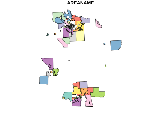
plot(st_as_sf(x %>% 
                dplyr::filter(!(AREANAME %LIKE% "Ca%" | AREANAME %LIKE% "Bi%")) %>% 
                dplyr::select(AREANAME, geom)))

Limitations

This is very largely format dependent, and by “format” we mean the driver as provided by GDAL.

We make no claims about performance or convenience, it will be affected by your system and your sf installation - lazysf just takes you closer the GDAL capabilities.

Performance can be excellent, and may be very competitive compared to reading an entire data source layer into memory. Really good drivers include ESRI Shapefile, Geopackage, PostgreSQL/PostGIS, MapInfo File, ESRI FileGDB, but there are dozens to choose from.

A query on a CSV, GeoJSON, or KML file (local or remote) is entirely subject to the performance of the matching GDAL driver.

Real DBs don’t have these special OGRSQL features, but they do have their own special syntax which for the most part can be sent straight through.

When using dplyr verbs (filter(), select(), mutate(), transmute(), arrange(), left_join(), …) we are also subject to the rules of SQL translation. There are no specific ones provided by lazysf but that might change.

Wrappers around lazysf could provide more specific tools for particular formats.

Can’t we just do this with sf’s query argument?

Yes (actually that is what lazysf uses) but with sf alone you get a fully materialized sf data frame, so you better get that query right first time!

With lazysf you get some control over intermediate steps, potentially expensive queries will only be run for a preview of the data until you are ready to fetch it.

Installation

remotes::install_github("mdsumner/lazysf")

Example

library(lazysf)
f <- system.file("gpkg/nc.gpkg", package = "sf", mustWork = TRUE)

## specify only the data source
lazysf(f)
#> # Source:   table<nc.gpkg> [?? x 15]
#> # Database: SFSQLConnection
#>     AREA PERIMETER CNTY_ CNTY_ID NAME  FIPS  FIPSNO CRESS_ID BIR74 SID74 NWBIR74
#>    <dbl>     <dbl> <dbl>   <dbl> <chr> <chr>  <dbl>    <int> <dbl> <dbl>   <dbl>
#>  1 0.114      1.44  1825    1825 Ashe  37009  37009        5  1091     1      10
#>  2 0.061      1.23  1827    1827 Alle… 37005  37005        3   487     0      10
#>  3 0.143      1.63  1828    1828 Surry 37171  37171       86  3188     5     208
#>  4 0.07       2.97  1831    1831 Curr… 37053  37053       27   508     1     123
#>  5 0.153      2.21  1832    1832 Nort… 37131  37131       66  1421     9    1066
#>  6 0.097      1.67  1833    1833 Hert… 37091  37091       46  1452     7     954
#>  7 0.062      1.55  1834    1834 Camd… 37029  37029       15   286     0     115
#>  8 0.091      1.28  1835    1835 Gates 37073  37073       37   420     0     254
#>  9 0.118      1.42  1836    1836 Warr… 37185  37185       93   968     4     748
#> 10 0.124      1.43  1837    1837 Stok… 37169  37169       85  1612     1     160
#> # … with more rows, and 4 more variables: BIR79 <dbl>, SID79 <dbl>,
#> #   NWBIR79 <dbl>, geom <MULTIPOLYGON [°]>

## specify the data source and a query to run
lazysf(f, query = "SELECT AREA, FIPS, geom FROM \"nc.gpkg\" WHERE AREA < 0.1")
#> # Source:   SQL [?? x 3]
#> # Database: SFSQLConnection
#>     AREA FIPS                                                               geom
#>    <dbl> <chr>                                                <MULTIPOLYGON [°]>
#>  1 0.061 37005 (((-81.23989 36.36536, -81.24069 36.37942, -81.26284 36.40504, -…
#>  2 0.07  37053 (((-76.00897 36.3196, -76.01735 36.33773, -76.03288 36.33598, -7…
#>  3 0.097 37091 (((-76.74506 36.23392, -76.98069 36.23024, -76.99475 36.23558, -…
#>  4 0.062 37029 (((-76.00897 36.3196, -75.95718 36.19377, -75.98134 36.16973, -7…
#>  5 0.091 37073 (((-76.56251 36.34057, -76.60424 36.31498, -76.64822 36.31532, -…
#>  6 0.072 37181 (((-78.49252 36.17359, -78.51472 36.17522, -78.51709 36.46148, -…
#>  7 0.053 37139 (((-76.29893 36.21423, -76.32423 36.23362, -76.37242 36.25235, -…
#>  8 0.081 37189 (((-81.80622 36.10456, -81.81715 36.10939, -81.82231 36.15786, -…
#>  9 0.063 37143 (((-76.48053 36.07979, -76.53696 36.08792, -76.5756 36.10266, -7…
#> 10 0.044 37041 (((-76.68874 36.29452, -76.64822 36.31532, -76.60424 36.31498, -…
#> # … with more rows

## specify the data source and the table/layer to access
lazysf(f, layer = "nc.gpkg") %>% 
  dplyr::select(AREA, FIPS, geom) %>% 
  dplyr::filter(AREA < 0.1)
#> # Source:   lazy query [?? x 3]
#> # Database: SFSQLConnection
#>     AREA FIPS                                                               geom
#>    <dbl> <chr>                                                <MULTIPOLYGON [°]>
#>  1 0.061 37005 (((-81.23989 36.36536, -81.24069 36.37942, -81.26284 36.40504, -…
#>  2 0.07  37053 (((-76.00897 36.3196, -76.01735 36.33773, -76.03288 36.33598, -7…
#>  3 0.097 37091 (((-76.74506 36.23392, -76.98069 36.23024, -76.99475 36.23558, -…
#>  4 0.062 37029 (((-76.00897 36.3196, -75.95718 36.19377, -75.98134 36.16973, -7…
#>  5 0.091 37073 (((-76.56251 36.34057, -76.60424 36.31498, -76.64822 36.31532, -…
#>  6 0.072 37181 (((-78.49252 36.17359, -78.51472 36.17522, -78.51709 36.46148, -…
#>  7 0.053 37139 (((-76.29893 36.21423, -76.32423 36.23362, -76.37242 36.25235, -…
#>  8 0.081 37189 (((-81.80622 36.10456, -81.81715 36.10939, -81.82231 36.15786, -…
#>  9 0.063 37143 (((-76.48053 36.07979, -76.53696 36.08792, -76.5756 36.10266, -7…
#> 10 0.044 37041 (((-76.68874 36.29452, -76.64822 36.31532, -76.60424 36.31498, -…
#> # … with more rows


## above was a real database (Geopackage), now with an actual shapefile
shp <- lazysf(system.file("shape/nc.shp", package = "sf", mustWork = TRUE))
library(dplyr)
shp %>%
 filter(NAME %LIKE% 'A%') %>%
 mutate(abc = 1.3) %>%
 select(abc, NAME, `_ogr_geometry_`) %>%
 arrange(desc(NAME))  #%>% show_query()
#> # Source:     lazy query [?? x 3]
#> # Database:   SFSQLConnection
#> # Ordered by: desc(NAME)
#>     abc NAME                                                    `_ogr_geometry_`
#>   <dbl> <chr>                                                      <POLYGON [°]>
#> 1   1.3 Avery    ((-81.94135 35.95498, -81.9614 35.93922, -81.94495 35.91861, -…
#> 2   1.3 Ashe     ((-81.47276 36.23436, -81.54084 36.27251, -81.56198 36.27359, …
#> 3   1.3 Anson    ((-79.91995 34.80792, -80.32528 34.81476, -80.27512 35.19311, …
#> 4   1.3 Allegha… ((-81.23989 36.36536, -81.24069 36.37942, -81.26284 36.40504, …
#> 5   1.3 Alexand… ((-81.10889 35.7719, -81.12728 35.78897, -81.1414 35.82332, -8…
#> 6   1.3 Alamance ((-79.24619 35.86815, -79.23799 35.83725, -79.54099 35.83699, …

# online sources can work
geojson <- file.path("https://raw.githubusercontent.com/SymbolixAU",
                      "geojsonsf/master/inst/examples/geo_melbourne.geojson")
lazysf(geojson)
#> # Source:   table<geo_melbourne> [?? x 8]
#> # Database: SFSQLConnection
#>    SA2_NAME polygonId SA3_NAME AREASQKM fillColor strokeColor strokeWeight
#>    <chr>        <int> <chr>       <dbl> <chr>     <chr>              <int>
#>  1 Abbotsf…        70 Yarra        1.74 #440154   #440154                1
#>  2 Albert …        59 Port Ph…     4.67 #450457   #450457                1
#>  3 Alphing…        41 Darebin…     2.89 #46075A   #46075A                1
#>  4 Armadale        66 Stonnin…     2.18 #460A5D   #460A5D                1
#>  5 Ascot V…        44 Essendon     3.84 #460C5F   #460C5F                1
#>  6 Brunswi…        36 Brunswi…     5.14 #472D7B   #472D7B                1
#>  7 Brunswi…        37 Brunswi…     2.17 #472D7B   #472D7B                1
#>  8 Brunswi…        38 Brunswi…     3.18 #472E7C   #472E7C                1
#>  9 Carlton         48 Melbour…     1.82 #443A83   #443A83                1
#> 10 Carlton…        71 Yarra        2.30 #443A83   #443A83                1
#> # … with more rows, and 1 more variable: `_ogr_geometry_` <POLYGON [°]>

DSN <- glue::glue("PG:host='{host}' dbname='{dbname}' user='{user}' password='{password}'")

dbConnect(SFSQL(), DSN)

but the same can be done with generic DBI and (for example) the Rpostgres package. With SFSQL() we just know that it’s executed by GDAL (via sf).

Some drivers are related

Note that GDAL drivers can be confusing, and it can be important to see the behaviours GDAL will provide by default. Here see that we can read from a Geopackage file but not as it was intended. We have used the driver-prefix to make GDAL choose its SQLite driver rather than the Geopackage driver.

library(lazysf)
gpkgfile <- system.file("gpkg/nc.gpkg", package = "sf", mustWork = TRUE)
lazysf(glue::glue("SQLite:{gpkgfile}"))
#> # Source:   table<gpkg_contents> [?? x 10]
#> # Database: SFSQLConnection
#>   table_name data_type identifier description last_change         min_x min_y
#>   <chr>      <chr>     <chr>      <chr>       <dttm>              <dbl> <dbl>
#> 1 nc.gpkg    features  nc.gpkg    ""          2016-09-28 14:57:13 -84.3  33.9
#> # … with 3 more variables: max_x <dbl>, max_y <dbl>, srs_id <int>

Code of Conduct

Please note that the lazysf project is released with a Contributor Code of Conduct. By contributing to this project, you agree to abide by its terms.