harrietr:
An R package for various phylogenetic and evolutionary
biology data manipulationsharrietr:Harriet is believed to be Charles Darwin’s pet giant
turtle. It is thought that Harriet spent the latter part of her life
at in Brisbane, Australia. Thus, Harriet satisfies the three criteria to
name this package: (1) it is somehow evolutionarily related; (2) it has
an Australian connection; and (3) it avoids the prefix
phylo used by many R evolutionarily- relavant
packages. The appended r just helps differentiate to make
it easier to search in Google, and aludes to the fact that it is related
to the programming language R.
Add Bioconductor to your list of default
repositories:
setRepositories(ind = 1:2)
Install harrietr:
install.packages("harrietr", dependencies = TRUE)
You must use devtools:
If you don’t have devtools installed:
install.packages('devtools')
Add Bioconductor to your list of default
repositories:
setRepositories(ind = 1:2)
Install harrietr:
devtools::install_github("andersgs/harrietr")
Three functions are provided at this time:
dist_long — This function takes as input an alignment in
DNA.bin format calculates all the pairwise distances, and
returns all the unique pairwise distances as a data.frame
in a long format. For example, in the case of three samples:
| id1 | id2 | distance |
|---|---|---|
| sample1 | sample2 | dist_12 |
| sample1 | sample3 | dist_13 |
| sample2 | sample3 | dist_23 |
You can give dist_long a tree (object of class
phylo), and it will add a fourth column with the pairwise
distance obtained from the tree:
| id1 | id2 | distance | evol_dist |
|---|---|---|---|
| sample1 | sample2 | dist_12 | evol_dist_12 |
| sample1 | sample3 | dist_13 | evol_dist_13 |
| sample2 | sample3 | dist_23 | evol_dist_23 |
melt_dist — This function is used by
dist_long, but it takes as input a distance matrix. This
might be useful if you alredy have a distance matrix that is imported
into R.
get_node_support — This function is written to work with
trees generated by IQTREE. In
particular, if the tree was generated when calculating node support by
both ultrafast bootstrap and SH approximate likelihood ratio test,
IQTREE writes the support as the node label in the Newick file in the
following format: "SH-aLRT/uBS". In other words, it is a
string with two values separated by a slash. The first
value is the SH-aLRT support (as a percentage) and the
second value is the ultrafast bootstrap support (also as a
percentage).
The output is a data.frame with each row representing an
internal node, with information that can be used to plot support
information layers on a tree.
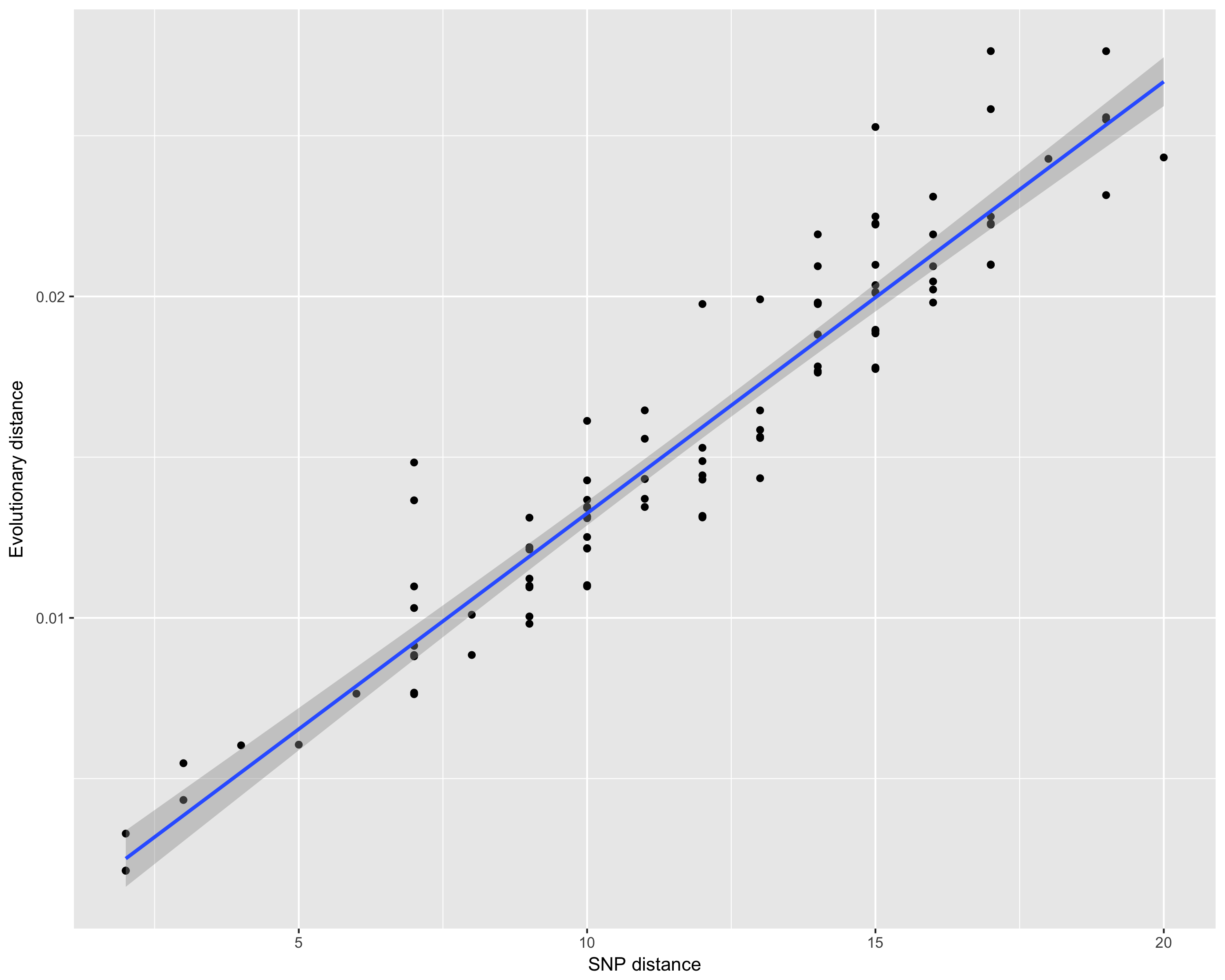
Assume you have a tree, and you want to understand what is the
relationship between the branch lengths and the number of SNPs. The
function dist_long can help you get there:
library(harrietr)
library(ggplot2)
data("woodmouse")
data("woodmouse_iqtree")
dist_df <- dist_long(aln = woodmouse, order = woodmouse_iqtree$tip.label, dist = "N", tree = woodmouse_iqtree)
ggplot(dist_df, aes(x = dist, y =  evol_dist)) +
  geom_point() + stat_smooth(method = 'lm') +
  ylab("Evolutionary distance") +
  xlab("SNP distance")
This will produce the following image:

Assume you have generated your ML tree with IQTREE, and wish to plot
it in R, and indicate which nodes have 50% or more support
values for both metrics (note: the value of 50% is
likely too low, these values are chosen only for illustration purposes).
The function get_node_support can help you get there:
library(ggtree)
library(dplyr)
library(harrietr)
data("woodmouse_iqtree")
p1 <- ggtree(woodmouse_iqtree)
node_support <- get_node_support(woodmouse_iqtree)
p1 +
  geom_point(data = node_support %>% dplyr::filter(`SH-aLRT` >= 50 & uBS >= 50), aes(x = x, y = y), colour = 'darkgreen', size = 3) +
  geom_point(data = node_support %>% dplyr::filter(`SH-aLRT` >= 50 & uBS >= 50), aes(x = x, y = y), colour = 'darkgreen', size = 5, pch = 21) +
  geom_point(data = node_support %>% dplyr::filter(`SH-aLRT` >= 50 & uBS >= 50), aes(x = x, y = y), colour = 'darkgreen', size = 7, pch = 21)
This will produce the following image:

Assume you have classified your samples into different groups (say A,
B, and C). These could be anything (e.g., MLST, sample source, host,
etc.), and you want summary information among and between the groups
(e.g., IQR, min/max dist). You can use dist_long and
add_metadata to generate the data.frame you
need:
library(ggplot2)
library(dplyr)
library(harrietr)
data("woodmouse")
data("woodmouse_iqtree")
data("woodmouse_meta")
dist_df <- dist_long(aln = woodmouse, order = woodmouse_iqtree$tip.label, dist = "N", tree = woodmouse_iqtree)
dist_df <- add_metadata(dist_df, woodmouse_meta, isolate = 'SAMPLE_ID', group = 'CLUSTER', remove_ind = TRUE)
dist_df %>%
  dplyr::group_by(CLUSTER) %>%
  dplyr::summarise(q50 = median(dist),
  q25 = quantile(dist, prob = c(0.25)),
  q75 = quantile(dist, prob = c(0.75)),
  min_dist = min(dist),
  max_dist = max(dist)) %>%
  ggplot( aes( x = CLUSTER, y = q50)) +
  geom_errorbar( aes(ymin = q25, ymax = q75),width = 0.25 ) +
  geom_point(size = 3, colour = 'darkred') +
  geom_point( aes( y = min_dist), colour = 'darkgreen', size = 3) +
  geom_point( aes( y = max_dist), colour = 'darkgreen', size = 3) +
  ylab("Pairwise SNP difference") +
  xlab("Groups")
This will produce the following image:
