
Leaf angle distribution (LAD) is an important factor for
characterizing the optical features of vegetation canopies (Ross
1981). It influences several processes such as photosynthesis,
evapotranspiration, spectral reflectance and absorptance (Vicari et al.
2019). LAD influence on radiation transmission is also described by
the leaf projection function (also known G-function), which is the
projection coefficient function of unit foliage area on a plane
perpendicular to the viewing direction (Ross
1981). Both parameters are therefore crucial to indirectly estimate
Leaf Area Index (LAI) from gap fraction or radiation trasmission
measurements.
Despite its importance, LAD is one of the most poorly characterized
parameters due to the difficulty of directly measure leaf inclination
angles, particularly in tall trees . As alternative to direct manual
measurements, Ryu et al.
(2010) proposed a robust and simple leveled photographic method to
measure leaf inclination angles, which was proven comparable to manual
clinometer measurements (Pisek et al.
(2011)).
Using this leveled photographic method, some dataset of leaf inclination
angle distributions have been compiled by some authors (Pisek et al.
2013; Raabe et al.
2015; Chianucci
et al. 2018; Pisek and Adamson
2020).
In this article we presented “LAD”, an R package to calculate the Leaf angle distribution (LAD) function and the G-function from measured leaf inclination angles.
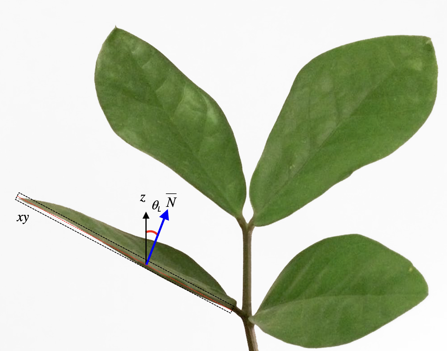
The method proposed by Ryu et al. (2010) consists of acquiring leveled images of the canopy using a digital camera. As some species may display phototropism, leaves shall be measured in all the azimuth directions and along the vertical profile of the surrounding canopy. Crowns of trees can be observed using towers, extendable poles, ladder, nearby tall buildings, or unmanned aerial vehicles (McNeil et al. 2016). The measurement of leaf inclination angle requires the identification of the leaf plane, from which the leaf normal is measured (Fig. 1). For this reason, the leaves must be selected from those oriented approximately parallel to the viewing direction of the camera (i.e., the leaves shown as a line in the image, Fig. 1), avoiding bended leaves to be measured.

Figure 1. Example of leaf inclination angle measurements from leveled photography. The measure of leaf inclination angle requires the identification of a hypothetical leaf plane xy, from which the leaf surface normal \(\hat{N}\) is calculated with respect to the zenith (z). In a 2-D space, such as a digital image, the only measurable leaf normal is that oriented perpendicular to the camera viewing direction, since the leaf inclination plane is parallel to the leaves (the red dashed line on the left side of the figure). From Chianucci et al. 2018, modified
Once a reliable set of leaf inclination angles measurements \(\theta_L\) are taken (a minimum of 75 measurements per species are recommended by Pisek et al. (2013)), two parameters \(\mu,\nu\) are derived for fitting a Beta distribution:
\(\mu=(1-\overline{t})(\frac{\sigma_0^2}{\sigma_t^2}-1)\)
\(\nu=\overline{t}(\frac{\sigma_0^2}{\sigma_t^2}-1)\)
where \(\sigma_0^2\) and \(\sigma_t^2\) are the maximum standard deviation and variance of t, respectively, and are calculated following Wang et al.(2007):
\(\sigma_0^2=\overline{t}(1-\overline{t})\)
\(\sigma_t^2=var(t)\)
with \(t=2\theta_L/\pi\), and \(\theta_L\) expressed as radians.
The two \(\mu,\nu\) parameters were then used to fit a Beta distribution function to represent the LAD of the considered canopy Goel and Strebel (1984):
\(f(t)=\frac{1}{B(\mu,\nu)}(1-t)^{\mu-1}t^{\nu-1}\)
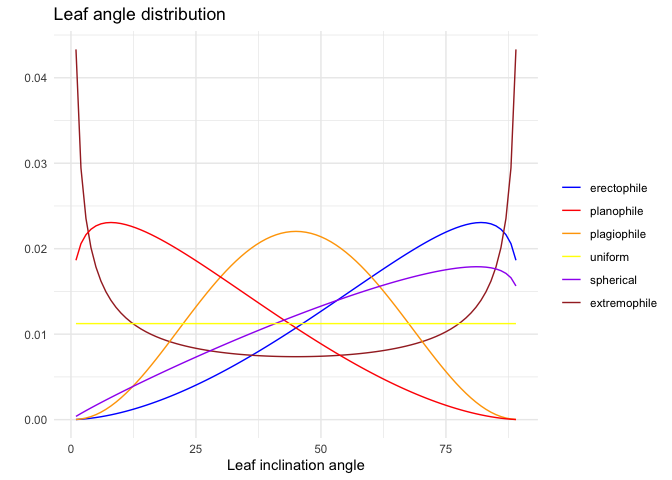
Following de Wit (1965), LAD functions can be described using six common functions based on empirical evidence of the natural variation of leaf normal distributions and mathematical considerations:
In spherical canopies, the relative frequency of leaf inclination angle is the same as for a sphere; planophile canopies are dominated by horizontally oriented leaves; plagiophile canopies are dominated by inclined leaves; erectophile canopies are dominated by vertically oriented leaves; extremophile canopies are characterized by both horizontally and vertically oriented leaves; uniform canopies are characterized by equal proportion of leaf inclination angles for any angle.

The fitted LAD function can then be compared with these six distributions, to determine the actual distribution type. The distribution type is classified using a leaf inclination index (Ross (1975)):
\(\chi^2=min\int_0^2\vert{f(\theta_L)-f_{deWit}(\theta_L)}\vert\)
The LAD function can also be used to calculate the G-function (Ross (1981)), which corresponds to the fraction of foliage area on a plane perpendicular to the view angle \(\theta\):
\(G(\theta)=\int_0^{2\pi}A(\theta,\theta_L)f(\theta_L)d\theta_L\),
where:
\(A(\theta,\theta_L) = \begin{cases} cos\theta\times{cos\theta_L} &\text{if } \vert{cot\theta \times{cot\theta_L}}\vert >1 \\ cos\theta\times{ cos\theta_L} [1+(2/\pi)(tan\psi-\psi)] &\text{if } \vert{cot\theta \times{cot\theta_L}}\vert \le{1} \end{cases}\)
and:
\(\psi=cos^{-1}(cot\theta\times{ cot\theta_L})\)
You can install the development version of LAD from GitLab using
devtools (Wickham et al. 2021):
# install.packages("devtools")
devtools::install_gitlab("fchianucci/LAD")
The package have two key functions to calculate LAD, G-function, summary leaf inclination angle statistics:
fitLAD calculates the LAD function and G-function from two-parameters \(\mu,\nu\) of Beta distribution.
The functions returns a list with two elements:
plot allows to display the
calculated LAD and G from measured leaf inclination angles.Example of graphical output:
fitLAD(4,2,plot=T)
The calcLAD(dataframe,angles,type,...) function allows
to calculate either summary leaf inclination angle statistics or the LAD
function and G-function from leaf inclination angle measurements. Three
important considerations must be drawn when using this function:
type.We will illustrate the function usage with example data from Chianucci et al. (2018), which represents the largest leaf inclination angle dataset for 138 temperate and boreal woody species.
head(Chianucci)## N ICP_Code Family Genus Species Author_citation
## 1 1 <NA> Araliaceae Eleutherococcus sessiliflorus (Rupr. & Maxim.) S.Y.Hu
## 2 2 <NA> Araliaceae Eleutherococcus sessiliflorus (Rupr. & Maxim.) S.Y.Hu
## 3 3 <NA> Araliaceae Eleutherococcus sessiliflorus (Rupr. & Maxim.) S.Y.Hu
## 4 4 <NA> Araliaceae Eleutherococcus sessiliflorus (Rupr. & Maxim.) S.Y.Hu
## 5 5 <NA> Araliaceae Eleutherococcus sessiliflorus (Rupr. & Maxim.) S.Y.Hu
## 6 6 <NA> Araliaceae Eleutherococcus sessiliflorus (Rupr. & Maxim.) S.Y.Hu
## Canopy_sector Angle_degree Date
## 1 whole canopy 20.973 11-10-11
## 2 whole canopy 34.472 11-10-11
## 3 whole canopy 7.787 11-10-11
## 4 whole canopy 1.868 11-10-11
## 5 whole canopy 52.667 11-10-11
## 6 whole canopy 65.433 11-10-11The calcLAD() function requires selecting the columns
with the leaf inclination angle measurements data (in degrees), the type
of calculations to be performed (‘summary’ or
‘extended’) and the grouping column(s).
By selecting type='extended' the function calculate LAD
function (pdf) and G-function (G) for each group:
calcLAD(Chianucci,Angle_degree,type='extended',Genus,Species)## # A tibble: 12,282 × 5
## Genus Species theta pdf G
## <chr> <chr> <int> <dbl> <dbl>
## 1 Acacia dealbata 1 0.0116 0.688
## 2 Acacia dealbata 2 0.012 0.688
## 3 Acacia dealbata 3 0.0123 0.688
## 4 Acacia dealbata 4 0.0125 0.687
## 5 Acacia dealbata 5 0.0126 0.686
## 6 Acacia dealbata 6 0.0127 0.685
## 7 Acacia dealbata 7 0.0128 0.684
## 8 Acacia dealbata 8 0.0128 0.683
## 9 Acacia dealbata 9 0.0129 0.682
## 10 Acacia dealbata 10 0.0129 0.68
## # ℹ 12,272 more rowsBy selecting type='summary' the function calculate mean
statistics (mean leaf inclination angle (MTA); standard deviation (SD),
frequency (NR), Beta parameters (mu,nu) and distribution type):
calcLAD(Chianucci,Angle_degree,type='summary',Genus,Species)## Joining with `by = join_by(Genus, Species)`
## Joining with `by = join_by(Genus, Species)`
## # A tibble: 138 × 8
## Genus Species MTA SD N mu nu distribution
## <chr> <chr> <dbl> <dbl> <int> <dbl> <dbl> <chr>
## 1 Acacia dealbata 40.9 24.5 283 1.27 1.06 uniform
## 2 Acer burgerianum 63.7 13.7 115 2.33 5.64 erectophile
## 3 Acer campestre 50.1 15.0 75 3.51 4.4 plagiophile
## 4 Acer griseum 33.6 20.9 80 2.09 1.24 planophile
## 5 Acer miyabei 44.9 15.5 80 3.72 3.71 plagiophile
## 6 Acer monspessulanum 20.1 14.8 105 4.21 1.21 planophile
## 7 Acer negundo 59.4 17.5 114 1.68 3.26 erectophile
## 8 Acer platanoides 26.8 16.7 1254 3.56 1.51 planophile
## 9 Acer pseudoplatanus 33.8 17.1 102 3.44 2.07 planophile
## 10 Acer rubrum 30.3 16.1 1001 3.98 2.03 planophile
## # ℹ 128 more rowsThe package was carried out within the Agritech National Research Center and received funding from the European Union Next-GenerationEU (National Recovery and Resilience Plan (NRRP) – MISSION 4 COMPONENT 2, INVESTMENT 1.4 – D.D. 1032 17/06/2022, CN00000022). This manuscript reflects only the authors’ views and opinions, neither the European Union nor the European Commission can be considered responsible for them.
Chianucci, F., Pisek, J., Raabe, K., Marchino, L., Ferrara, C. and Corona, P., 2018. A dataset of leaf inclination angles for temperate and boreal broadleaf woody species. Annals of Forest Science, 75(2), pp.1-7., doi: https://doi.org/10.1007/s13595-018-0730-x
De Wit, C., 1965. Photosynthesis of leave canopies. Center for Agricultural Publication and Documents, Wageningen, The Netherlands.
Goel, N.S. and Strebel, D.E., 1984. Simple beta distribution representation of leaf orientation in vegetation canopies 1. Agronomy Journal, 76(5), pp.800-802, doi: https://doi.org/10.2134/agronj1984.00021962007600050021x.
McNeil BE, Pisek J, Lepisk H, Flamenco EA, 2016. Measuring leaf angle distribution in broadleaf canopies using UAVs. Agric For Meteorol 218-219:204–208, doi: https://doi.org/10.1016/j.agrformet.2015.12.058.
Pisek, J. and Adamson, K., 2020. Dataset of leaf inclination angles for 71 different Eucalyptus species. Data in brief, 33, p.106391. doi: https://doi.org/10.1016/j.dib.2020.106391.
Pisek, J., Ryu, Y. and Alikas, K., 2011. Estimating leaf inclination and G-function from leveled digital camera photography in broadleaf canopies. Trees, 25(5), pp.919-924, doi: https://doi.org/10.1007/s00468-011-0566-6.
Pisek, J., Sonnentag, O., Richardson, A.D. and Mõttus, M., 2013. Is the spherical leaf inclination angle distribution a valid assumption for temperate and boreal broadleaf tree species. Agricultural and Forest Meteorology, 169, pp.186-194, doi: https://doi.org/10.1016/j.agrformet.2012.10.011.
Raabe K, Pisek J, Sonnentag O, Annuk K, 2015. Variations of leaf inclination angle distribution with height over the growing season and light exposure for eight broadleaf tree species. Agric For Meteorol 21:2–11, doi: https://doi.org/10.1016/j.agrformet.2015.07.008.
Ross, I. and Ross, J., 1981. The radiation regime and architecture of plant stands (No. 3). Springer Science & Business Media.
Ross, J., 1975. Radiative transfer in plant communities. Vegetation and the Atmosphere, pp.13-55.
Ryu, Y., Sonnentag, O., Nilson, T., Vargas, R., Kobayashi, H., Wenk, R. and Baldocchi, D.D., 2010. How to quantify tree leaf area index in an open savanna ecosystem: a multi-instrument and multi-model approach. Agricultural and Forest Meteorology, 150(1), pp.63-76, doi: https://doi.org/10.1016/j.agrformet.2009.08.007.
Vicari M.B., Pisek J., Disney M., 2019. New estimates of leaf angle distribution from terrestrial LiDAR: Comparison with measured and modelled estimates from nine broadleaf tree species, Agricultural and Forest Meteorology, 264:322-333, doi: https://doi.org/10.1016/j.agrformet.2018.10.021.
Wang, W.M., Li, Z.L. and Su, H.B., 2007. Comparison of leaf angle distribution functions: Effects on extinction coefficient and fraction of sunlit foliage. Agricultural and Forest Meteorology, 143(1-2), pp.106-122, doi: https://doi.org/10.1016/j.agrformet.2006.12.003.
Wickham, H., Hester, J., Chang, W., Bryan, J., 2021. devtools: Tools to Make Developing R Packages Easier.